Getting Started With Machine Learning

• 15 min read
• Process, Product Strategy, Experience Design, Machine Learning
• Share on Twitter, LinkedIn

About The Author

PhD in artificial intelligence at UC Berkeley, with a focus on small neural networks in perception, for autonomous vehicles. Big fan of cheesecake, corgis, and … More about Alvin ↬

Email Newsletter

Your (smashing) email

Weekly tips on front-end & UX.
Trusted by 200,000+ folks.

The goal of machine learning is to find patterns in data and use those patterns to make predictions. It can also give us a framework to discuss machine learning problems and solutions — as you’ll see in this article.

First, we will start with definitions and applications for machine learning. Then, we will discuss abstractions in machine learning and use that to frame our discussion: data, models, optimization models, and optimization algorithms. Later on in the article, we will discuss fundamental topics that underlie all machine learning methods and conclude with practical guidance for getting started with using machine learning. By the end, you should have an understanding of how to advance your practice and study of machine learning.

Let’s begin.

So, What Exactly Is Machine Learning?

Machine learning is generically a set of techniques to find patterns in data. Applications range from self-driving cars to personal AI assistants, from translating between French and Taiwanese to translating between voice and text. There are a few common applications of machine learning that already or could potentially permeate your day-to-day.

1. Detecting anomalies
   Recognize spikes in website traffic or highlight abnormal bank activity.
2. Recommend similar content
   Find products you may be looking for or even Smashing Magazine articles that are relevant.
3. Predict the future
   Plan the path of neighboring vehicles or identify and extrapolate market trends for stocks.

The above are few of many applications of machine learning, but most applications tie back to learning the underlying distribution of data. A distribution specifies events and probability of each event. For example:

• With 50% probability, you buy an item $5 or less.
• With 25% probability, you buy an item $5-$10.
• With 24% probability, you buy an item $10-100.
• With 1% probability, you buy an item > $100.

Using this distribution, we can accomplish all of our tasks above:

1. Detecting anomalies
   With a $100 purchase, we can confidently call this an anomaly.
2. Recommend similar content
   A purchase of $3 means we should recommend more items $5 or less.
3. Predict the future
   Without any prior information, we can predict that the next purchase will be $5 or less.

With a distribution of data, we can accomplish a myriad of tasks. In sum, one goal in machine learning is to learn this distribution.

Even more generically, our goal is to learn a specific function with particular inputs and outputs. We call this function our model. Our input is denoted x. Say our model, which accepts input x, is

f(x) = ax

Here, a is a parameter of our model. Each parameter corresponds to a different instance of our model. In other words, the model where a=2 is different from the model where a=3. In machine learning, our goal is to learn this parameter, changing it until we do “well.” How do we determine which values of a do “well”?

We need to define a way to evaluate our model, for each parameter a. To start, the output of f(x) is our prediction. We will refer to y as our label, meaning the true and desired output. With our predictions and our labels, we can define a loss function. One such loss function is simply the difference between our prediction and our label, |f(x) - y|. Using this loss function, we can then evaluate different parameters for our model. Picking the best parameter for our model is known as training. If we have a few possible parameters, we can simply try each parameter and pick the one with the smallest loss!

However, most problems are not as simple. What happens if there are an infinite number of different parameters? Let’s say all decimal values between 0 and 1? Between 0 and infinity? This brings us to our next topic: abstractions in machine learning. We will discuss different facets of machine learning, to compartmentalize your knowledge into data, models, objectives, and methods of solving objectives. Beyond learning the right parameter, there are plenty of other challenges: how do we break down a problem as complex as controlling a robot? How do we control a self-driving car? What does it mean to train a model that identifies faces? The section below will help you organize answers to these questions.

Abstractions

There are countless topics in machine learning — at various levels of specificity. To better understand where each piece fits in the larger picture, consider the following abstractions for machine learning. These abstractions compartmentalize our discussion of machine learning topics, and knowing them will make it easier for you to frame topics. The following classifications are taken from Professor Jonathan Shewchuck at UC Berkeley:

1. Application and Data
   Consider the possible inputs and the desired output for the problem.
   

   Questions: What is your goal? How is your data structured? Are there labels? Is it reasonable for us to extract output from the provided inputs?
   
   Example: The goal is to classify pictures of handwritten digits. The input is an image of a handwritten number. The output is a number.

   
   
2. Model
   Determine the class of functions under consideration.
   

   Questions: Are linear functions sufficient? Quadratic functions? Polynomials? What types of patterns are we interested in? Are neural networks appropriate? Logistic regression?
   
   Example: Linear regression

   
   
3. Optimization Problem
   Formulate a concrete objective in mathematics.
   

   Questions: How do we define loss? How do we define success? Should we apply additionally penalties to bias our algorithm? Are there imbalances in the data our objective needs to consider?
   
   Example: Find `x` that minimizes |Ax-b|^2

   
   
4. Optimization Algorithm
   Determine how you will solve the optimization problem.
   

   Questions: Can we compute a solution by hand? Do we need an iterative algorithm? Can we convert this problem to an equivalent but easier-to-solve objective, and solve that one?
   
   Example: Take derivative of the function. Set it to zero. Solve for our optimal parameter.

   
   

Abstraction 1: Data

In practice, collecting, managing, and packaging data is 90% of the battle. The data contains samples in which each sample is a specific realization of our input. For example, our input may generically be images of dogs. The first sample is specifically a picture of Maxie, my Bernese Mountain dog-chow chow mix at home. The second sample is specifically a picture of Charlie, a young corgi.

While training your model, it is important to handle your data properly. This means separating our data accordingly and not peeking prematurely at any set of data. In general, our data is split into three portions:

1. Training set
   This is the dataset you train your model on. The model may see this set hundreds of times.
2. Validation set
   This is the dataset you evaluate your model on, to assess accuracy and tune your model or method accordingly.
3. Test set
   This is the dataset you evaluate on to assess accuracy, once at the very end. Running on the test set prematurely could mean your model overfits to the test set as well, so run only once. We will discuss the notion of “overfitting” in more detail below.

Abstraction 2: Models

Machine learning methods are split into the following two:

Supervised Learning

In supervised learning, our algorithm has access to labeled data. Still, we explore the following two classes of problems:

• Classification
  Determine which of k classes {C_1, C_2, ... C_k} to which each sample belongs, e.g. “Which breed of dog is this?” The dog could be one of {"corgi", "bernese mountain dog", "chow chow"...}
• Regression
  Determine a real-valued output (which are often probabilities), e.g. “What is the probability this patient has neuroblastoma (eye cancer)?”

Unsupervised Learning

In unsupervised learning, our algorithm does not have access to labels, and we explore the following classes of problems:

• Clustering
  Cluster samples into k clusters. We do not have a label for the resulting clusters. “Which DNA sequences are most similar?”
• Dimensionality reduction
  Reduce the number of “unique” (linearly independent) features we consider. “What are common features of faces?”

Abstraction 3: Optimization Objective

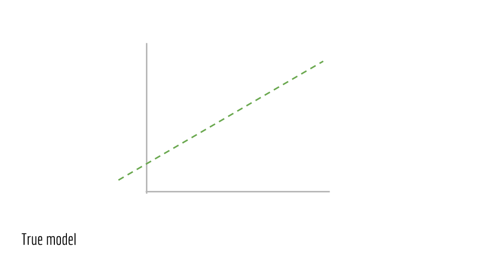
Before discussing optimization objectives and algorithms, we’ll need an example to discuss. Least squares are the canonical example. We will restrict our attention to a specific form of least squares: Let us return to our grade-school problem of fitting a line to some points.

Let’s recall the equation of a line:

y = m * x + b

Assume we have such a line. This is the true underlying model.

Now, sample points from this line.

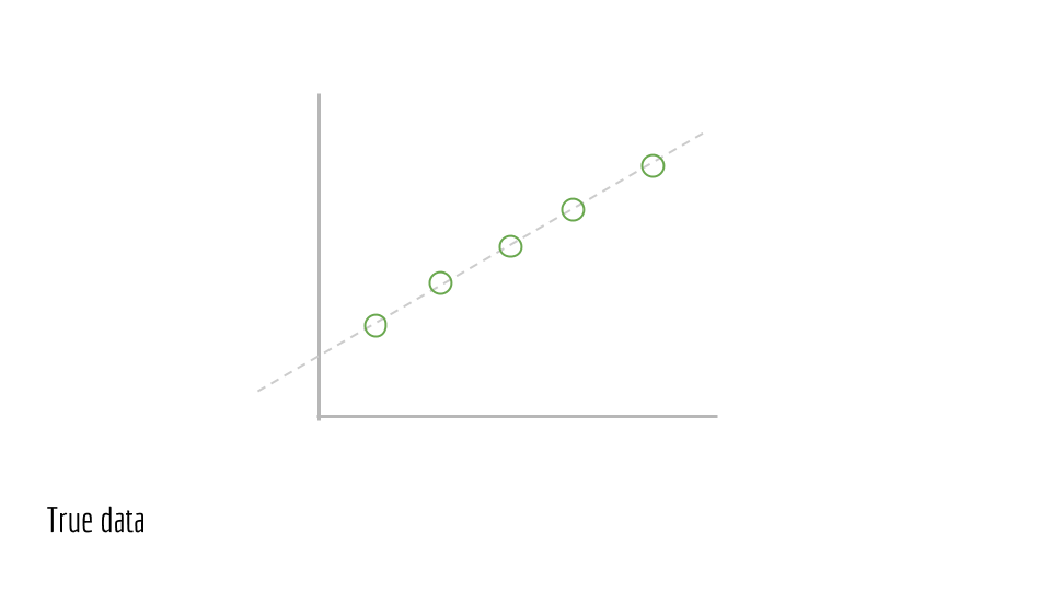
For each point, jiggle it a little bit. In other words, add noise, which is random perturbations. This noise is due to real-world processes.

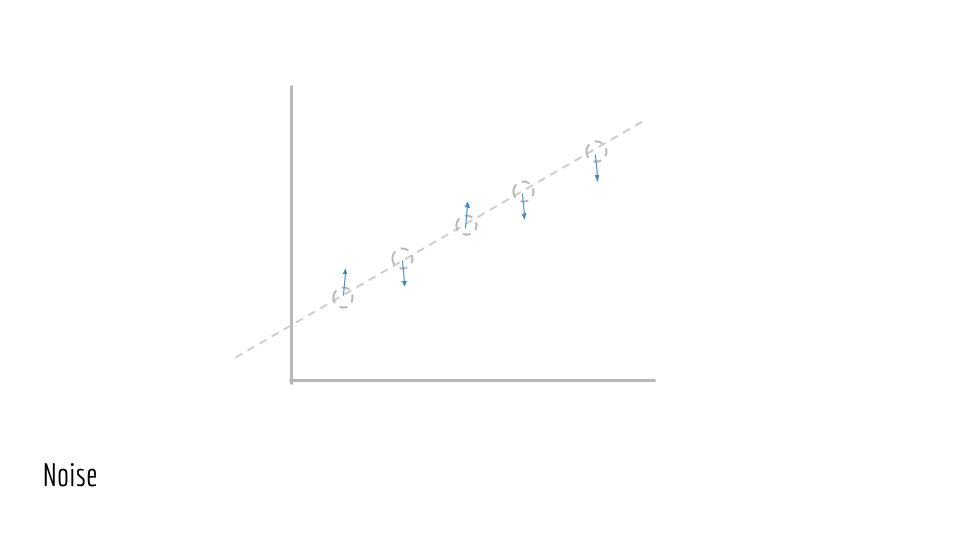
This gives us our observed data. We will call these points (x_1, y_1), (x_2, y_2), (x_3, y_3).... This is the training data we are given to train a model on. We do not have access to the underlying line that generated this data (the original green line).

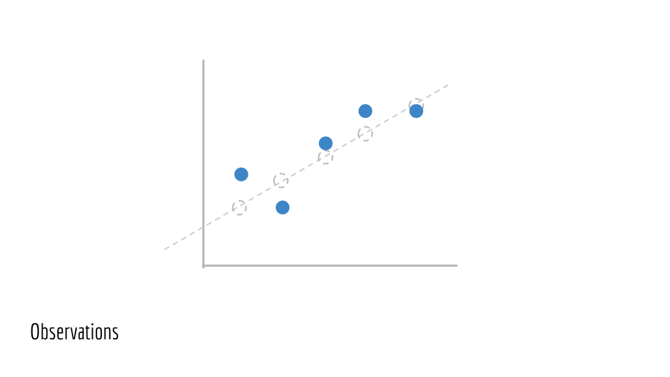
Say we have an estimate for the parameters of a line. In this case, the parameters are m and b. This gives us a predicted line, drawn in blue below.

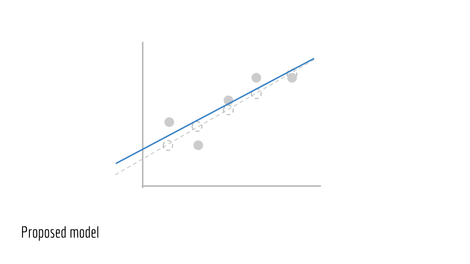
We wish to evaluate our blue line, to see how accurate it is. To start, we use m and b to estimate y. We compute a set of ŷ values.

ŷ_i = m * x_i + b

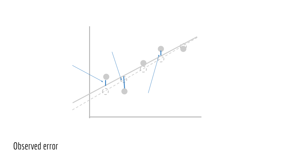
The error for a single predicted ŷ_i and true y_i is simply

(ŷ_i−y_i)^2

Our total error is then the sum of squared differences, across all samples. This yields our loss.

∑(ŷ_i−y_i)^2

Presented visually, this is the vertical distance between our observed points and our predicted line.

Plugging in ŷ_i from above, we then have the total error in terms of m and b.

∑(m * x_i + b − y_i)^2

Finally, we want to minimize this quantity. This yields our objective function, abstraction 3 from our list of abstractions above.

min_{m, b} ∑(m * x_i + b−y_i)^2

The above states in mathematics that the goal is to minimize the loss by changing values of m and b. The purpose of this section was to motivate fitting a line of best of fit, a special case of least squares. Additionally, we showed examined the least squares objective. Next, we need to solve this objective.

Abstraction 4: Optimization Algorithm

How do we minimize this? We take the derivative with respect to m`, set to 0 and solve. After solving, we obtain the analytical solution. Solving for an analytical solution was our optimization algorithm, the fourth and final abstraction in our list of abstractions.

Note: The important portion of this section is to inform you that least squares have a closed form solution, meaning that the optimal solution for our problem can be computed, explicitly. To understand why this is significant, we need to examine a problem without a closed-form solution. For example, we could never solve x=logx for a standard base-10 logarithm. Try graphing these two lines, and we see that they never intersect. In which case, we have no closed-form solution. On the other hand, ordinary least squares have a closed-form — which is good news. For any problem reduced to least squares, we can then compute the optimal solution, given our data and assumptions.

Fundamental Topics

Before studying more methods, it is necessary to understand the undercurrents of machine learning. These will govern the initial study of machine learning:

Bias-Variance Tradeoffs

One of machine learning’s most dreaded evils is overfitting in which a model is too closely tailored to the training data. In the limit, the most overfit model will memorize the data. This might mean that if one does well on exam A, one repeats every detail for exam B — down to the duration of an inter-exam restroom trip and whether or not one used the urinal.

A related but less common evil is underfitting, where the model is not sufficiently expressive to capture important information in the data. This could mean that one looks only at homework scores to predict exam scores, ignoring the effects of reading notes, completing practice exams, and more. Our goal is to build a model that generalizes to new examples while making the appropriate distinctions.

Given these two evils, there are a variety of approaches to fighting both. One is modifying your optimization objective to include a term that penalizes model complexity. Another is tuning hyperparameters that govern either your objective or your algorithm, which may correspond to notions such as “training speed” or “momentum.” The bias-variance tradeoff gives us a precise way of defining and handling both overfitting and underfitting.

Maximum Likelihood Estimation (MLE) + Maximum A Posteriori (MAP)

Say we have ice cream flavors A, B, and C. We observe different recipes. Our goal is to predict which flavor each recipe produces.

One way to predict flavors based on recipes is to first estimate the following probability:

P(flavor|recipe)

Given this probability and a new recipe, how can we predict the flavor? Given a recipe, simply consider the probability of each of the flavors A, B, C.

P(flavor=A|recipe) = 0.4
P(flavor=B|recipe) = 0.5
P(flavor=C|recipe) = 0.1

Then, pick the flavor that has the highest probability. Above, flavor B has the highest probability, given our recipe. Thus, we predict flavor B. Restating the above rule in mathematics, we have:

argmax_{flavor} P(flavor|recipe)  # argmax means take the flavor that corresponds to the max value

However, the only information at our disposal is the reverse: the probability of some recipe given the flavor.

P(recipe|flavor)

For Maximum Likelihood Estimates, we make assumptions and find that the two values are proportional.

P(recipe|flavor) ~ P(flavor|recipe)

Since we’re only interested in the class with maximum probability P(flavor|recipe), we can simply find the class with maximum probability, for a proportional value P(recipe|flavor).

argmax_{flavor} P(recipe|flavor)

MLE offers the above objective as one way to predict, using the probability of data given the labels.

However, allow me to convince you that it’s reasonable to assume we have (x|y). We can estimate this from observed, real-world data. For example, say we wish to estimate the number of marbles each student in your class carries, based on the number of rubber ducks the student carries.

Each student’s number of rubber ducks is the data x, and the number of marbles she or he has is y. We will use this sample data below.

| x | y |
|---|---|
| 1 | 2 |
| 1 | 1 |
| 1 | 2 |
| 2 | 1 |
| 2 | 2 |
| 1 | 2 |

For every y, we can compute the number of x, given us P(x|y). For the first one, P(x=1|y=1), consider all of the rows where y=1. There are 2, and only one of them has x=1. Therefore, P(x=1|y=1) = 1⁄2. We can repeat this for all values of x and y.

P(x=1|y=1) = 1/2
P(x=2|y=1) = 1/2
P(x=1|y=2) = 3/4
P(x=2|y=2) = 1/4

Featurizations, Regularization

Least squares draw lines of best fit for us. Note that least squares can fit the model anytime the model is linear in its inputs x and outputs y.

Say m=1. We have the following equation:

y = x + b

However, what if we had data that doesn’t generally follow a line? Specifically, consider a set of data sampled along a circle. Recall that the equation for a circle is:

x^2 + y^2 = r^2

Can least squares fit this well? As it stands, no. The model is not linear in its inputs x and outputs y. Instead, the model above is quadratic in x and y. However, it turns out that we can use still use least squares, just with a modification. To accomplish this, we featurize our samples.

Consider the following: what if the input to our model was x_ = x^2 and y_ = y^2? Then, our model is trying to learn the following model.

x_ + y_ = r^2

Is this linear in the model’s input x_ and output y_? Yes. Note the subtlety. The current model is still quadratic in x,y but it is linear in x_,y_. This means that least squares can fit the data if we square x^2 and y^2 before training least squares.

More generally, we can take any non-linear featurization to apply least squares to labels that are non-linear in the features. This is a fairly powerful tool, known as featurization.

However, featurizations lead to more complex models. Regularization allows us to penalize model complexity, ensuring that we do not overfit the training data.

Conclusion

In this article, you’ve touched on major topics in the fundamentals of machine learning. Using the abstractions above, you now have a framework to discuss machine learning problems and solutions. Using the fundamental topics above, you now also have quintessential concepts to learn more about, giving you the necessary tools to evaluate risk and other concerns in a machine learning application.

Other Resources

We will continue to explore these topics in depth, both the undercurrents of machine learning and specific methods. In the interim, here are resources to further your study and exploration of machine learning:

• “Introduction to Machine Learning,” Machine Learning course CS189, UC Berkeley
• NumPy (for efficient linear algebra utilities)
• scikit-learn (for out-of-the-box machine learning methods)

Further Reading

• The Impact Of Agile Methodologies On Code Quality
• Crafting Experiences: Uniting Rikyu’s Wisdom With Brand Experience Principles
• Powerful Image Analysis With Google Cloud Vision And Python
• Using Friction As A Feature In Machine Learning Algorithms

(ra, il, mrn)